An Alternative to Statistical Significance for Making Decisions with Experiments

For a long time in experimentation, the way we’ve made decisions is by using statistical significance (stat sig.) However, there are alternative approaches which are rapidly gaining adoption. In this article we will compare the stat sig approach with the one that most big tech companies are moving toward (and which we use at LaunchDarkly.)

There are various ways to use statistical significance in online experimentation. The most recent formulations use a method called sequential testing which allows you to run the experiment until you achieve statistical significance and then make that treatment (aka variation, aka arm) of your experiment the new default for all of your target users. You might also hear this referred to as null hypothesis significance testing (NHST).

Recently, more and more experimentation systems are moving away from statistical significance (Facebook’s Ax, Google Optimize, etc.). It turns out that while statistical significance does help you reduce false positives, it also misses a lot of valuable gains. The trade off when reducing false positives is more false negatives.

While previously we used stat sig because it was “scientific,” more and more we are seeing this is not actually true. The Stanford Encyclopedia of Philosophy entry on Decision Theory puts it this way:

As we see in the quote above, the alternative to stat sig is expected utility. For online experimentation, the key difference between stat sig and expected utility is that stat sig has a goal of controlling Type I (false positive) and Type II (false negative) error rates over all experiments. Expected utility, on the other hand, has the goal of making the best decision for each experiment given the evidence.

For a good overview in making decisions based on expected utility check out this great video from the New York Times: "Making Choices Like a Poker Champ."

This will be important to keep in mind as we compare statistical significance and expected utility. Since their goals are different, they will do better or worse depending on how you measure them.

Typically, in online experimentation, our goal is to make the best decision, and it is easy to show that stat sig does not result in the best decision in many cases. Another approach we could take is to look at the loss for the different methods. For this article we’ll just look at the count of correct and incorrect decisions. Let’s dive in.

A typical A/B test

In this section, we’ll look at a common type of experiment you see in the digital world. We have the status quo and we’ll introduce a contender for some feature area. Let’s say that we think the landing page for our marketing site can be improved to increase sales in our e-commerce store.

What we typically do in this case is design a new version of a landing page and run an experiment where we measure revenue. Let’s see what designing an experiment and running it might look like under the two frameworks. We’ll call our existing design "Treatment A" and our new design "Treatment B."

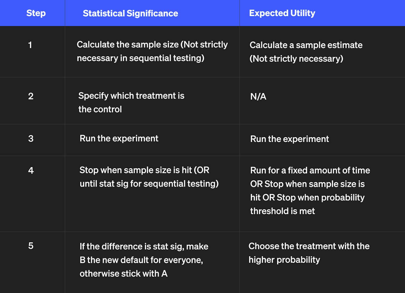
Under a statistical significance framework you would typically do the following:

Line 5 is where we find the decision points. Notice the key difference is that in stat sig, you need a significant amount of evidence against "A" in order to select "B." By contrast, in the expected utility approach you just pick whichever has the most evidence in its favor.

Just to make that super clear, let’s imagine the data we saw during the experiment looked like this:

If this was the outcome, then notice that both the stat sig and the expected utility approaches would have the same verdict: launch B to all your users. This is because for the stat sig approach, B is statistically significant, and for the expected utility approach, B is higher than A. So B satisfies the requirements under both approaches.

What if the outcome was slightly different? Imagine it looked like this:

In this scenario, the two decision-making frameworks differ in their recommendation. Although the data shows that B is better than A, stat sig says there’s not enough data to make that determination so you should keep A. Expected utility, on the other hand, says you should go with B, because the evidence that B is better is greater than the evidence that A is better.

It turns out that if you use the expected utility decision-making method, then across all your decisions you’ll garner more value for the business.

What about Type I and Type II errors?

Type I (false positive) and Type II (false negative) errors are something that we aim to control when using stat sig. If we calculate a sample size, we can specify our desired Type II error rate and then when we run the experiment we can specify our desired Type I error rate. Unfortunately, as much as we might desire otherwise, the error rates must be greater than 0.

With expected utility, we don’t try to control for error rates because that’s not our goal. Our goal is to pick the treatment that provides the most business value. It might seem like we’re missing something or that we might make more mistakes, but with a little perspective we can see why we’re not.

Let’s start with a Type I error. It’s a false positive. That is a case where we pick the treatment, but it was actually not different from the control. But notice if there’s no difference, then you can’t make a mistake if your goal is to pick the treatment with the most value, because either option satisfies that requirement (when there’s a tie for value, expected utility shows us that both options are equally good decisions). Either choice is optimal as long as there are no switching costs. Imagine two stocks will perform equally well over the next year; if that’s true then it doesn’t matter which stock you invest in. (Naturally you might then think that stat sig is better when there are switching costs. We’ll cover why that’s not necessarily true in another post.)

Now onto Type II errors: the way that stat sig controls the false negative rate, i.e., the percentage of times that you will not see stat sig even when there is a change, is using a sample size calculator. With a large enough sample size you can see any size effect. But with small samples you can only get statistical significance with very large effects.

Notice that with expected utility we are not trying to detect certain effect sizes. We just want to make the right decision. This is what’s happening in the second example table in the previous section. It’s not stat sig because the effect size is too small for the sample size. But we can still see that it’s likely to be the best and we should choose it.

Nonetheless, just like with stat sig, if we want more confidence we could collect more data. In future posts we’ll talk about cases when we might want to do so. But for most experiments, we should just be selecting the treatment that is most likely to be best.

Simulating the two approaches

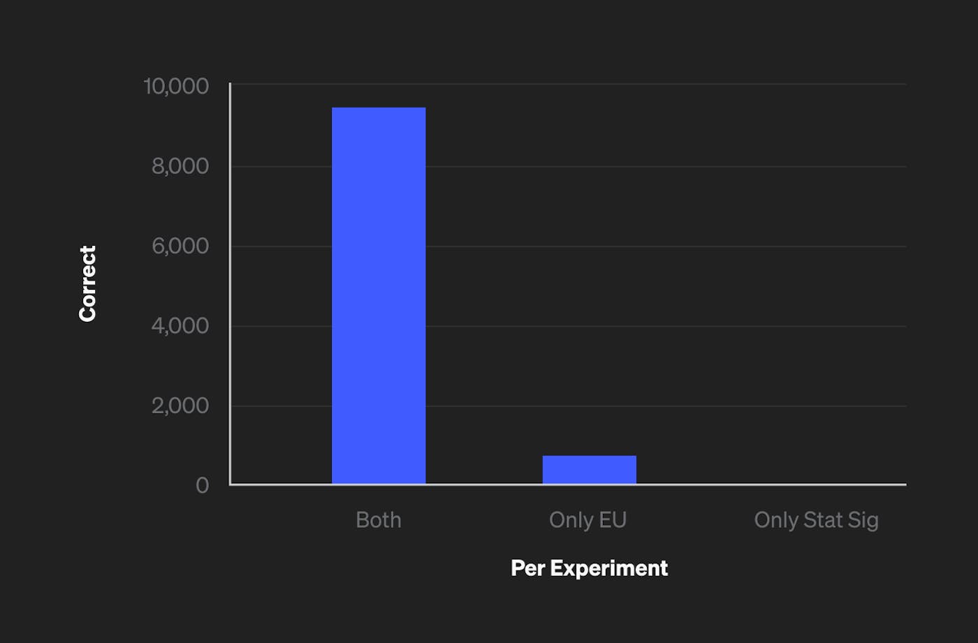
Here is a Scala notebook simulating many experiments, with and without differences between treatments, and comparing the different decision-making methods. You’ll notice that the expected utility method for making decisions performs better when the goal is to pick the best option. Here’s an example output from the notebook showing how many times stat sig and expected utility get the same, correct result, how many times only expected utility gets the correct result, and how many times only stat sig gets the correct result.

We see here that expected utility results in the same, correct decision in all the cases that statistical significance does, plus additional cases where stat sig would result in the incorrect decision.

In this particular simulation, the percentage of correct outcomes for stat sig and expected utility are 93.94% and 99.05% respectively. Again, we are taking "correct" to mean that we picked the better option or, in the case of no difference, picked an equally good option.

This was a fairly high-level overview. There are interesting scenarios where you might think one approach is better than another. Or you might want to view this under another lens, like loss functions. For now we hope that you have gained a new perspective on the different ways you can make decisions in experimentation.

References

Test & Roll: Profit-Maximizing A/B Tests

Stanford Encyclopedia of Philosophy “Decision Theory”