Covariate adjustment and CUPED methodology

Overview

This guide explains the methodology and usage of CUPED (Controlled experiments Using Pre-Experiment Data) for covariate adjustment in LaunchDarkly Experimentation results.

Covariate adjustment refers to the use of variables unaffected by treatment, known as covariates, for:

• Variance reduction: reduces the variance of experiment lift estimates, which increases measurement precision and experiment velocity.
• Bias removal: removes the conditional bias of experiment lift estimates, which increases measurement accuracy.

In mainstream statistics, covariate adjustment is typically performed using Fisher’s (1932) analysis of covariance (ANCOVA) model. In the context of online experimentation, Deng et al. (2013) introduced CUPED (short for Controlled Experiments Using Pre-Experiment Data), which can be thought of as a special case of ANCOVA with the pre-period version of the modeled outcome as a single covariate.

In this guide, we use the terms covariate adjustment, analysis of covariance (ANCOVA), and CUPED interchangeably.

Context

In a randomized experiment, there are three types of variables defined for each experiment unit, such as “user,” in a user-randomized experiment:

• Treatment: a variable indicating treatment for the unit. For example: 1 if the unit is assigned to the “treatment” variation, and 0 if assigned to the “control” variation.
• Outcomes: post-treatment variables that we want to measure experiment performance on, such as experiment revenue.
• Covariates: pre-treatment variables that we use to improve our measurement of the outcomes, typically for segmentation and variance reduction, such as pre-experiment revenue.

Outcomes are post-treatment variables. These are variables potentially affected by the treatment, or measured after the treatment is assigned. An example is revenue measured after the user enters the experiment.

Covariates must be pre-treatment variables, which are variables measured before the treatment is assigned, or variables unaffected by treatment. Examples include revenue measured before a user enters the experiment, which is measured before treatment, and gender, which is unaffected by the treatment.

Method

The goal of covariate adjustment is to improve the measurement of an experiment outcome, such as experiment revenue, through the use of prognostic covariates. Prognostic covariates are covariates predictive of the outcome. Pre-experiment revenue is an example of a prognostic covariate, which is typically predictive of experiment revenue. The ANCOVA model, and CUPED in particular, does this by leveraging the correlation, which is the strength of linear relationship, between an outcome and a set of covariates, with the goal of improving measurement precision and accuracy.

Variance Reduction

We illustrate this with a simple example of an outcome $Y$, such as experiment revenue, and a covariate $X$, such as pre-experiment revenue.

In this example, there is a strong linear relationship between them for both treatment and control variations, shown in the scatter plot on the left below:

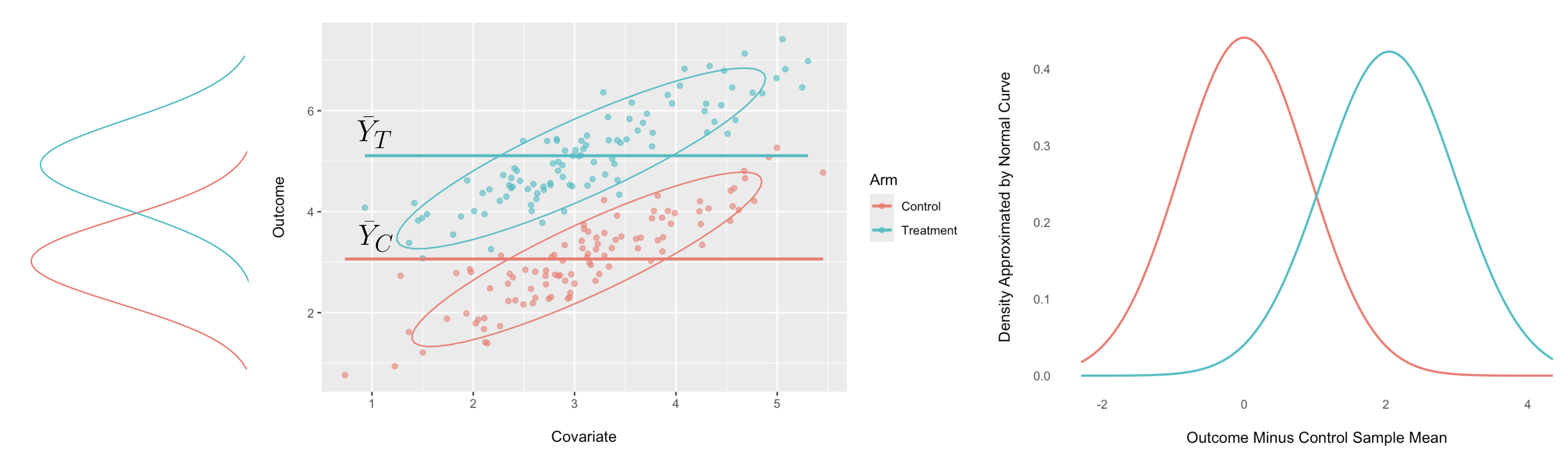
Predicting the observations in the treatment and control variations with, respectively, the sample means $\bar{Y}_T$ and $\bar{Y}_C$ results in a large variance for the errors, as illustrated in the plot on the right above.

However, we can leverage the linear relationship between $Y$ and $X$ by predicting the observations in the treatment and control variations with, respectively, the regression predictions $\hat{Y}_T = \hat{\alpha}_T + \hat{\beta}_T X$ and $\hat{Y}_C = \hat{\alpha}_C + \hat{\beta}_C X$, as shown in the scatter plot on the left below:

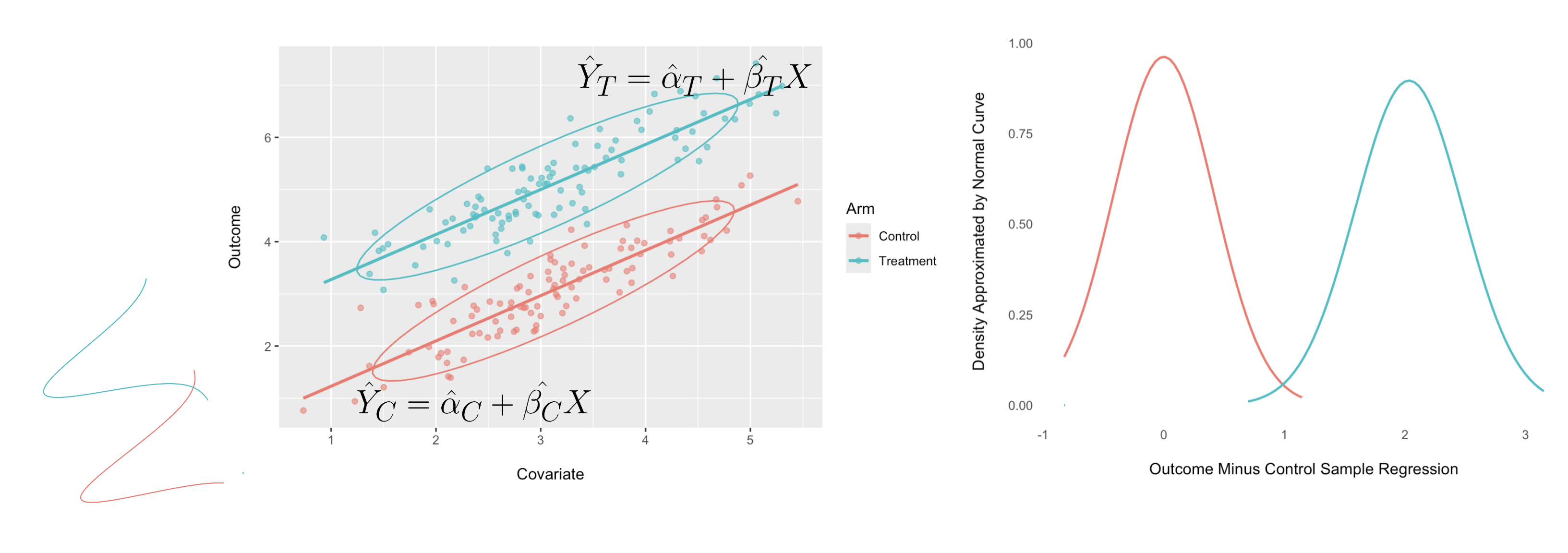
This results in smaller variance for the errors, as shown in the density plot on the right above. The above two scatter plots were inspired by those shown in Huitema (2011).

The correlation, which is the strength of the linear relationship between the outcome $Y$ and the covariate $X$, determines how much the error variance is reduced. The larger the correlation, the larger the variance reduction.

Specifically, if we denote the original error variance estimates for the two variations by, respectively, $s_T^2$ and $s_C^2$, and the new error variance estimates using CUPED by, respectively, $s_{T, CUPED}^2$ and $s_{C, CUPED}^2$, and the outcome-covariate correlations by, respectively, $r_T$ and $r_C$, then the following holds approximately:

The proportional reduction in error variance is approximately the square of the correlations:

If the correlations in both variations are $60\%$, the error variance will be reduced by $60\%^2 = 36\%$, and if they are $70\%$, the error variance will be reduced by $70\%^2 = 49\%$. The proportional reduction in the error variance translates to about the same proportion reduction in the variance of the experiment lift estimate, which translates to the same proportional reduction in experiment duration on average. Therefore, when the correlations are $60\%$, the experiment duration will be reduced by as much as $36\%$ on average, and when they are $70\%$, the experiment duration will be reduced by as much as $49\%$ on average. In other words, this can cut experiment duration nearly in half.

Bias Removal

In addition to reducing the variance of lift estimates, CUPED applies an adjustment to the sample means $\bar{Y}_T$ and $\bar{Y}_C$ to produce the following covariate-adjusted means:

Where $\bar{X}_T$ and $\bar{X}_C$ denote the covariate means for, respectively, the treatment and control variations, and $\bar{X}_{all}$ denote the covariate mean over all experiment variations. Although the unadjusted means $\bar{Y}_T$ and $\bar{Y}_C$ are unbiased estimators of the variation averages over many realizations of the experiment, for a specific experiment there could be some conditional bias. Conditional bias may occur due to the random imbalances between the treatment and control variation covariate means $\bar{X}_T$ and $\bar{X}_C$. As long as the linear regression model is correct, the adjustments $- \hat{\beta_T} \left(\bar{X}_T - \bar{X}_{all} \right)$ and $- \hat{\beta_C} \left(\bar{X}_C - \bar{X}_{all} \right)$ control for these imbalances and remove the conditional bias.

Implementation

In this section we discuss the scope and model for the CUPED implementation in the LaunchDarkly Experimentation product.

CUPED availability

CUPED is available for experiments when the following criteria have been met:

• Average metrics: CUPED can be applied to metrics using the “average” analysis method, including conversion metrics and continuous numeric metrics. CUPED is not applied to metrics using a percentile analysis method.
• Metrics with historical data: CUPED can only be applied to a metric that has received events within the seven days prior to the start of the experiment. This is because CUPED requires historical metric data to compare current metric data to.
• Unfiltered metrics: CUPED cannot be applied to metrics with event filters.
• Experiments that have been running for at least 90 minutes: CUPED is not available for experiments receiving events for less than an hour and a half, due to the longer time it takes to compute the covariate-adjusted means and their standard errors (SEs) in the data pipeline. Results before the first hour and a half are not covariate-adjusted, even if the above CUPED criteria have been met.

Model

The covariate adjustment model implemented is characterized by the following two features:

• Feature 1—Most General Model: LaunchDarkly uses the most general ANCOVA model, which allows for unequal covariate slopes and unequal error variances by experiment group. Using the convention of Yang and Tsiatis (2001), we refer to this model as the ANCOVA 3 model. To learn more, read Covariate adjustment.
• Feature 2—Single Pre-period Covariate: LaunchDarkly restricts the model to use only one covariate. We used the pre-period version of the modeled outcome, which is the covariate proposed by Deng et al. (2013) for the CUPED model and by Soriano (2019) for the PrePost model.

Besides giving us the most general model, another advantage of Feature 1 is that we can implement the ANCOVA model by fitting separate linear regression models by variation. This means we fit one for each experiment variation, which simplifies implementation. One advantage of Feature 2 is that we can fit the linear regression models using simple analytical formulas without needing to use specialized statistical software for linear regression. Combining Features 1 and 2 yields a very simple SQL implementation that you can apply to big data with computational efficiency.

Some may express concern about our using only one covariate in the model when we could potentially include more. In practice, using only the single pre-period covariate is advantageous from both the data collection and model fit points of view:

• Data collection: it simplifies the data collection process because we do not need to gather more covariates. Instead, we only need to collect data for the current outcome in the pre-period to obtain the pre-period covariate.
• Model fit: in practice, the pre-period covariate used is typically the covariate with the largest correlation with the experiment-period outcome. When such a highly correlated covariate is included in the model, including additional covariates typically does not improve the overall fit. In other words, the R-squared of the linear regression model would not increase by much.

The pre-period covariate is measured over a seven-day lookback window before the start of the experiment. Precedent for using only seven days is established by the implementation of the PrePost model for covariate adjustment for YouTube experiments, mentioned in Soriano (2019), which is the basis for our implementation.

There is also a tradeoff between using shorter versus longer windows in terms of relevance versus sufficiency. Shorter windows may have more relevance due to the recency of the information measured, but may not have captured all the information to optimize the outcome-covariate correlation. Longer windows capture more information, but risk including irrelevant information from older events, which may decrease the outcome-covariate correlation.

CUPED on the Results tab

Each LaunchDarkly experiment indicates whether CUPED is enabled or disabled on its Results tab above the “Exposures” graph.

The CUPED statuses indicate:

• CUPED Disabled: CUPED is disabled for your experiment because all of its metrics are percentile metrics.
• CUPED Enabled: If CUPED is enabled, the experiment can be in one of three states:
  • CUPED is enabled, but no metrics are covariate-adjusted yet. This can be because the experiment has been receiving results for less than 90 minutes, or because there is no pre-experiment data in the seven days before the experiment started.
  • Only some of the metrics are covariate-adjusted.
  • All of the metrics are covariate-adjusted.

Advanced topics

For those interested, we will cover some advanced topics in the following sections.

Covariate adjustment

For a two-variation experiment, you can formulate the ANCOVA 3 model implemented at LaunchDarkly as a single model. For example:

where $A = T$ if unit $i$ is in the treatment variation and $A = C$ if unit $i$ is in the control variation.

The original ANCOVA model introduced by Fisher (1932) makes the following assumptions:

• Assumption 1—Equal Slopes: equal covariate slope $\beta_A$ for all experiment variations, that is, $\beta_T = \beta_C$ in the example above.
• Assumption 2—Equal Variances: equal error variance $\sigma_A^2$ for all experiment variations, that is, $\sigma_T^2 = \sigma_C^2$ in the example above.

Yang and Tsiatis (2001) referred to this original model as the ANCOVA 1 model. If we remove Assumption 1 to allow for unequal covariate slopes, that is, allowing for $\beta_T \neq \beta_C$, then we have what Yang and Tsiatis (2001) calls the ANCOVA 2 model, also known as Lin’s (2013) model or the ANHECOVA (ANalysis of HEterogeneous COVAriance) model of Ye et al. (2021).

However, in practice it can be convenient to relax Assumption 2 in addition to Assumption 1, which allows for unequal error variances, that is, $\sigma_T^2 \neq \sigma_C^2$. This gives us what we call the ANCOVA 3 model.

This can be implemented in two ways:

• Single model: a single generalized least squares (GLS) model, which allows for error variances that vary by experiment group. This can be fitted using, for example, the nlme::gls function in R.
• Separate models: an equivalent, but simpler, way to implement ANCOVA 3 is to fit one separate regression model for each experiment variation.

Fitting separate models has the advantage of fitting very simple regression models when there is only one covariate. This makes for a simple SQL implementation without leveraging additional software, which improves computational efficiency, especially on big data. We give an example of a simple SQL implementation of the ANCOVA 3 model in the section SQL Implementation.

Causal inference

In a comparative study, whether a randomized experiment or an observational study, the goal is to perform causal inference, which includes estimating the causal effect of a treatment, for example, the causal effect of a new product feature on revenue.

Under the Neyman-Rubin potential outcomes framework for causal inference, we begin with individual potential outcomes (IPOs) $Y_i\left(1 \right)$ and $Y_i\left(0 \right)$ for, respectively, receiving the treatment and not receiving the treatment, for each individual $i$. The individual treatment effect (ITE) for individual $i$ is given by:

One estimand for the causal effect of treatment is the average treatment effect (ATE), which is the average of the ITEs:

This is the difference between the average potential outcomes (APOs) $E \left( Y_i\left(1 \right) \right)$ and $E \left( Y_i\left(0 \right) \right)$ of receiving and not receiving the treatment, respectively. An alternate causal estimand is the relative average treatment effect (RATE):

In the LaunchDarkly Experimentation product, we estimate the APO $E \left( Y_i\left(a \right) \right)$ for each experiment variation $a$ for every combination of analysis time, experiment iteration, metric, and attribute. We then perform causal inference based on estimating the RATE for each treatment variation versus control.

Covariate-adjusted means

To perform causal inference, we first estimate the IPOs by their respective linear regression predictions for the treatment and control variations using the ANCOVA 3 model described earlier:

The APOs are estimated by averaging the IPOs over all available units. In this case, the units are in both the treatment and control variations:

where $\bar{X}$ denotes the average of the covariate over all units in both variations. Because the linear regression models have only one predictor, the estimated regression intercepts are given by:

Therefore, the estimated APOs are given by:

We refer to $\bar{Y}_{T, adj}$ and $\bar{Y}_{C, adj}$ as covariate-adjusted means. They are the unadjusted sample means $\bar{Y}_{T}$ and $\bar{Y}_{C}$, minus the adjustments $\hat{\beta}_T \left( \bar{X}_T - \bar{X}_{all} \right)$ and $\hat{\beta}_T \left( \bar{X}_C - \bar{X}_{all} \right)$. This removes conditional bias due to the randomized imbalances between the covariate means $\bar{X}_T$ and $\bar{X}_C$ for both the treatment and control variations, respectively.

You can compute the estimated regression slopes with the following formulas:

where:

• $s_{Y, T}$ and $s_{Y, C}$ are the sample standard deviation (SD) for the outcome in the treatment and control variations, respectively
• $s_{X, T}$ and $s_{X, C}$ are the sample SD for the covariate in the treatment and control variations, respectively, and
• $r_T$ and $r_C$ are the outcome-covariate correlation in the treatment and control variations, respectively.

We can show that the estimated SEs for the covariate-adjusted means for both the treatment and control variations are:

where $n_T$ and $n_C$ are the sample sizes for the treatment and control variations, respectively.

When the sample sizes $n_T$ and $n_C$ are large and the imbalances $\bar{X}_T - \bar{X}_{all}$ and $\bar{X}_C - \bar{X}_{all}$ are negligible, the above SEs reduce to the following:

Therefore, the proportional variance reduction for each is approximately equal to the squared correlation for the variation, as we showed earlier:

Frequentist and Bayesian approaches

For frequentist estimates, the estimates of the APOs are the above covariate-adjusted means $\bar{Y}_{T, adj}$ and $\bar{Y}_{C, adj}$. In the Bayesian model, the APO estimates are regularized using empirical Bayes priors. To learn more, read Statistical methodology for Bayesian experiments and Statistical methodology for frequentist experiments.

The Bayesian results without covariate adjustment through CUPED continue to use the normal-normal model for custom conversion count and custom numeric continuous metrics and the beta-binomial model for custom conversion binary, clicked or tapped, and page viewed metrics. However, the Bayesian results with covariate adjustment through CUPED will use the normal-normal model for all metrics using the “average” analysis method, including custom conversion binary metrics. Under this model, we assume the following prior distribution for the parameter estimated in variation $A_{T, C}$ :

For details on the prior mean $\mu_{0, A}$ and $\sigma_{0, A}^2$, read Statistical methodology for Bayesian experiments.

LaunchDarkly provides a frequentist estimate $\hat\theta_A$ and its estimated standard error $\hat{SE}\left(\hat\theta_A \right)$. For the non-CUPED results, the estimate is the sample mean. For CUPED results, the estimate in the covariate-adjusted mean $\hat\theta_A = \bar{Y}_{A, adj}$, with details provided in the previous section.

We define precision as the inverse of the variance, which is equivalent to the inverse of the squared standard error. Therefore, the estimated precisions of the prior distribution and the frequentist estimate are, respectively:

Define the following precision sum and weight:

Then the posterior distribution of the estimated parameter is given by:

where the posterior mean is given by the precision-weighted average of the frequentist estimate $\hat{\theta}$ and the prior mean $\mu_{0, A}$, and the posterior variance is the inverse of the sum of the frequentist estimate precision $Prec\left(\hat\theta_A \right)$ and the prior precision $Prec\left(\theta_{prior, A} \right)$.

SQL implementation

Here is an example SQL implementation of the ANCOVA 3 model for covariate adjustment to demonstrate its simplicity.

Assume that we have fields y and x in a table named UnitTable, which is aggregated by experiment units, with fields for analysis time, experiment, metric, segment, and variation. The following simple query produces non-CUPED and CUPED estimates with corresponding SEs aggregated by combinations of analysis time, experiment, metric, segment, and variation:

1
WITH BasicStats AS (
2
  SELECT
3
    analysis_time,
4
    experiment,
5
    metric,
6
    segment,
7
    arm,
8
    COUNT(*) AS n,
9
    AVG(y) AS ybar,
10
    AVG(x) AS xbar,
11
    AVG(x) OVER (PARTITION BY analysis_time, experiment, metric, segment)
12
      AS xbar_all,
13
    STDEV_SAMP(y) AS s_y,
14
    STDEV_SAMP(x) AS s_x,
15
    CORR(x, y) AS r
16
  FROM UnitTable
17
  GROUP BY 1, 2, 3, 4, 5
18
)
19
SELECT
20
  analysis_time,
21
  experiment,
22
  metric,
23
  segment,
24
  arm,
25
  'unadjusted' AS method,
26
  n AS exp_unit_count,
27
  ybar AS estimate,
28
  s_y / SQRT(n) AS estimate_std_error
29
FROM BasicStats
30
UNION ALL
31
SELECT
32
  analysis_time,
33
  experiment,
34
  metric,
35
  segment,
36
  arm,
37
  'covariate_adjusted' AS method,
38
  n AS exp_unit_count,
39
  ybar - (r * s_y / s_x) * (xbar - xbar_all) AS estimate,
40
  s_y * SQRT(1 - SQUARE(r)) * SQRT((n - 1) / (n - 2)) *
41
  SQRT(1 / n + SQUARE(xbar - xbar_all) / (SQUARE(s_x) * (n - 1)))
42
    AS estimate_std_error
43
FROM BasicStats

The BasicStats common table expression (CTE) produces the following aggregated statistics needed to compute the unadjusted and covariate-adjusted means for each combination of analysis time, experiment, metric, segment, and variation:

• Sample means: the sample means $\bar{Y}$ and $\bar{X}$ for the outcome and the covariate, respectively.
• Sample standard deviations: the sample standard deviations $s_Y$ and $s_X$ for the outcome and the covariate, respectively.
• Sample correlation: the sample correlation $r$ between the outcome and the covariate.

The outer query takes the aggregated statistics from the BasicStats CTE to compute the unadjusted and covariate-adjusted means and their SEs using the formulas we derived in the “Covariate-adjusted means” section.

References

Deng, Alex, Ya Xu, Ron Kohavi, and Toby Walker (2013). “Improving the Sensitivity of Online Controlled Experiments by Utilizing Pre-Experiment Data.” WSDM’13, Rome, Italy.

Fisher, Ronald A. (1932). Statistical Methods for Research Workers. Oliver and Boyd. Edinburgh, 4th ed.

Huitema, Bradley (2011). Analysis of Covariance and Alternatives: Statistical Methods for Experiments, Quasi-Experiments, and Single-Case Studies, 2nd ed. Wiley.

Lin, Winston (2013). “Agnostic Notes on Regression Adjustments to Experimental Data: Reexamining Freedman’s Critique.” Annals of Applied Statistics, 7(1): 295-318.

Soriano, Jacopo (2019). “Percent Change Estimation in Large Scale Online Experiments.” https://arxiv.org/pdf/1711.00562.pdf.

Yang, Li and Anastasios A. Tsiatis. (2001). “Efficiency Study of Estimators for a Treatment Effect in a Pretest-posttest Trial.” American Statistician, 55: 314-321.

Ye, Ting, Jun Shao, Yanyao Yi, and Qingyuan Zhao (2023). “Toward Better Practice of Covariate Adjustment in Analyzing Randomized Clinical Trials.” Journal of the American Statistical Association, 118(544): 2370-2382.