Feature Engineering in Machine Learning: Concepts & Workflow

In production machine learning, model performance often depends as much on feature engineering as on the algorithm itself. Consider a fraud detection system: Raw inputs such as transaction time, amount, device type, and location are rarely enough on their own. Features like transaction frequency, unusual spending patterns, or deviations from a user’s typical behavior often provide the signal a model needs to detect fraud accurately. Strong features can reveal meaningful patterns, while weak ones make it harder to separate signal from noise.

Feature engineering bridges raw data and model performance. It involves selecting, transforming, and encoding information so learning algorithms can use it effectively. In tabular machine learning, this often means creating derived variables, encoding categories, scaling numeric values, or aggregating behavior over time. In deep learning, feature engineering is usually less about manual feature creation and more about input representation, preprocessing, tokenization, and embeddings. Across both settings, it remains essential to build models that work well in practice.

Feature engineering best practices

In production systems, feature engineering relies on a set of best practices that ensure that features are correct, reproducible, and usable in both training and inference. For example, in a fraud detection pipeline, transaction events from payment services may first be aggregated into behavioral features such as transaction frequency, spending velocity, or location changes. These features are then kept in a feature store and used during model training. At inference time, the prediction service retrieves the same engineered features to ensure that the model receives inputs consistent with training. The practices discussed in this article help ensure that those features remain correct, reproducible, and operationally reliable.

Understand the data-generating process before engineering features

Strong feature engineering starts before transformations. Select features that reflect how the system actually generates data—such as instrumentation, business rules, and operational peculiarities—and use causal reasoning to determine what the model is permitted to know at prediction time. Without knowing how a value is created, when it is available, and which processes contribute to it, it can be very easy to generate features that look predictive when you are offline, but when you take it into production, it can leak, become biased, or be systematically missing. Causal awareness is used to differentiate between a stable signal and spurious correlations, which can fail under a distribution shift.

Build a data provenance map

Before applying any transformations, get clear on the source of each field. The same metric can imply a lot of different things based on the way it is gathered. For example, a field like failed_login_count in fraud detection might seem simple, but its origin (e.g., authentication service, analytics pipeline, or security tool with filters) determines its actual meaning. One source may include only failures entered by users, whereas another may be able to include blocked bot traffic or retries through mobile clients.

To understand a field's provenance, examine its origin and lifecycle: value producers, recording triggers, collection boundaries (inclusion/exclusion), data freshness (latency, delays, backfills), and definition stability over time.

Validate semantics and units, not just schemas

Most production failures come from incorrect assumptions about what the data represents. Check whether a field is used as a feature, verify units and timezone conventions, examine rounding behavior, and check whether values such as 0 or -1 are placeholders for missing data before using a field.

Also, verify what a metric is aggregated over, since “per user” can refer to different definitions across systems. Capture the field’s intended meaning, expected range, and missing-value interpretation in a short note alongside the transformation code.

Explicitly hunt for leakage and proxy variables

Features that are not available at prediction time are a common source of failure. Every feature should be testable by verifying that their values are known at prediction time and not derived from actions taken afterward. Post-decision fields and operational response variables are common offenders.

In training pipelines, use a per-example cutoff timestamp and compute features only from data available at or before that time, with rolling windows and event-log aggregates. Enforce point-in-time checks in the pipeline rather than relying on manual review.

Treat missingness as a signal and as a failure mode

Missing values can mean different things, e.g., “not applicable,” “not collected,” “dropped by a pipeline,” “intentionally withheld,” etc. Avoid collapsing all of these into one imputation rule. Include indicators of missingness of key fields and track missingness by group, as systematic missingness may also cause bias, weaken model calibration, and indicate collection regressions at an early stage.

The final test before deciding on a new feature is to ensure that it is available where and when required, that it will not leak in the long term, and that it does not have an apparent leakage path.

How to automate data cleaning and transformation pipelines

Manual preprocessing may work during exploration but can fail in production environments. A repeatable pipeline is essential for automating, versioning, and executing data cleaning and transformation procedures. This includes handling tasks like addressing missing values, standardizing units, and scaling. The goal is to ensure that the same input consistently yields the same output upon repeated execution.

Define preprocessing as code

Avoid implementing feature preprocessing logic in temporary notebooks or one-off scripts. Instead, define preprocessing as versioned, reusable code that runs consistently in both training and inference pipelines.

In the following example, the pipeline fills missing values, converts transaction amounts to a common currency, and scales age using precomputed parameters. Importantly, statistics such as age_mean and age_std should be fit on training data only and then reused unchanged during validation and inference to avoid leakage.

Separate fit and transform

Preprocessing parameters should be fit on training data and reused unchanged during validation and inference, and the learned parameters should be reused directly and identically. Preprocessing parameters include scaling statistics, vocabularies, category mappings, and imputation values. Version these artifacts and update them alongside the model.

Use pipelines, not scripts

Preprocessing is often performed in a special-purpose pipeline of features but not as a local script in production. Orchestrators and distributed engines, like Airflow, Kubeflow, and Spark, are commonly used in batch pipelines to provide scheduling, retries, lineage, and scalability.

Make transformations consistent across training and serving

Training-serving skew often results from duplicated or inconsistent transformation logic. Define transformations once and reuse them in both training and inference. Use a shared transformation code, shared artifacts, or a feature store that imposes the same definitions. Let quality checks become operational.

Construct features using domain knowledge

Construct features that capture real-world behavior rather than relying on raw attributes. Derived variables such as ratios, time intervals, and aggregates often reflect underlying system dynamics (e.g., user intent, risk accumulation, or recency effects) more effectively than raw inputs. In practice, aggregates and ratios that are carefully selected work better than further complexity in models.

Prioritize behavior over raw attributes

Static fields are often weak proxies for the outcome you want to predict. Behavioral features capture how an entity changes over time and often provide stronger signals than static attributes. These features can drift quickly in dynamic environments and must be monitored in production.

Common high-signal behavioral patterns include:

• Recency (time since the last event)
• Frequency (counts over trailing windows)
• Intensity (rates such as events per session or spend per day)
• Monotonic progression (cumulative totals or trend deltas)
• Normalization ratios that remove scale effects

Use time-aware constructions instead of raw timestamps

Raw timestamps are rarely useful on their own. Convert timestamps into recency, intervals, or windowed aggregates aligned with the prediction task.

Here, average_spend summarizes spending behavior per session, while days_since_purchase turns a raw date into a recency feature that is often more predictive than the timestamp itself.

Guard ratios and aggregations

Ratios and aggregates require guardrails in production. Denominators should be protected with floors or conditional logic, missingness indicators should be added where values may be absent, aggregation windows must be explicitly defined and kept consistent, and event time should not be confused with processing time.

Keep features serving-feasible

Check that the complex constructions can be calculated in the environment where the predictions will be done before investing. If the online inference is unable to access the necessary joins or history, then compute with a batch, save the output to a feature store, or rearchitect the feature to make use of available signals.

Encode and scale input data appropriately

Encode and scale input data based on cardinality, model requirements, and serving constraints. The wrong encoding choice can introduce leakage, increase latency, or create unstable features in production.

Choose encoding based on cardinality and serving constraints

Choose encoding strategies based on cardinality, drift behavior, and interpretability needs. The appropriate method depends on category cardinality, drift patterns, and interpretability requirements:

• Low cardinality: One hot encoding is easy and debuggable.
• High cardinality: Look to frequency based encoding, hashing, or embeddings to avoid sparse blowups.

Use target encoding carefully

Target encoding can be useful, but a naive implementation can leak label information. If category means are computed on the full dataset, each row is encoded using its own target and information from validation or test examples, which can severely inflate offline performance. For that reason, target encoding should be computed with out-of-fold logic during training and then applied to new data using the mappings learned from the training set.

The following example shows the basic idea, but it should not be used directly on the full dataset in practice.

In production systems, target encoding should follow several safeguards. Encodings should be computed using training data only, and training rows should use out-of-fold computation to avoid leakage. Rare categories should be smoothed or regularized so they do not introduce unstable signals. The resulting category-to-value mapping should then be persisted as an artifact and include a defined fallback strategy for unseen categories at inference time.

Text features: match representation to latency and model type

For text inputs, the representation depends on model architecture and system constraints. TF IDF is a strong baseline for linear models and is generally not an issue in terms of latency. Embeddings based on word2vec offer a small vector representation and are likely to work well when the semantics of tokens are relevant. Sentence transformer embeddings capture richer semantics but require more compute and storage.

Scale numeric features with a consistent fit scope

Having numeric features on comparable scales enables many models to be trained and to act more predictably, particularly linear models and neural networks. In production, inconsistent scaling often shows up as unstable training, slow or failed convergence, and prediction drift when training and serving apply different statistics.

Standardization scales values based on a z-score transformation and is useful where a feature is approximately normally distributed. Min-max normalization puts values in a restricted range and is helpful when the natural scale of the feature matters. Robust scaling uses the median and interquartile range and performs better when outliers would otherwise distort scaled values. Lock encoding and scaling into versioned artifacts so training and inference consistently apply identical transformations.

Incorporate temporal and sequential signals correctly

Incorporate temporal signals using strict point-in-time correctness. To avoid leakage, all features must be computed using only information available at prediction time.

Use windows, lags, and intervals to encode dynamics

Time-based features are more effective when they capture behavioral changes rather than raw timestamps.

Common patterns include:

• Lag features referring to previous values (e.g., t-1, t-7)
• Rolling statistics computing values over trailing windows (e.g., moving average, sum, min, max)
• Recency features measure how recently an event occurred

Shift rolling features to avoid leakage

Rolling computations must exclude the current and future timestep if your serving path would not have that information.

For example, the shift below ensures that the feature at time t only uses values from times < t. Without it, offline training can quietly incorporate future information and inflate metrics.

Define the cutoff time explicitly

For each training example, define a prediction timestamp and compute all features relative to that cutoff. This eliminates peeking as a result of joins, late events, or backfills.

Handle late data and time semantics consistently

Actual pipelines are characterized by event lag and reprocessing. Choose between event time or processing time features, and use those choices consistently during training and serving. In case aggregates can be changed by late data, track feature freshness and define backfill policies. In streaming setups, define watermarks or late-data tolerance thresholds so the system has a clear rule for when to finalize windows and how to handle events that arrive after the cutoff.

Select and reduce features based on system constraints

Apply feature selection only when it reduces training cost, serving latency, or overfitting risk. Many modern models tolerate redundant features, so selection should be driven by system constraints rather than default practice. The value of feature selection depends on dataset size, feature dimensionality, and model type. Aggressive pruning can remove weak but useful signals in large data regimes and may not be as productive as it seems as a way of simplifying things.

Prune when it reduces risk or cost

Feature selection becomes valuable when systems exhibit signals such as very high feature dimensionality that slows training or serving, strong multicollinearity or redundant signals, clear overfitting or unstable feature importance across runs, or operational fragility caused by too many upstream dependencies.

Use selection methods that match your constraints

Select methods based on data size, feature dimensionality, and system constraints. Correlation or variance filters are usually a naive initial step to eliminate constant or extremely redundant features. In smaller sets of features, recursive feature elimination (RFE) can be used to find a succinct set of features that maintains the performance. In cases where the scale is important, model-based feature importance offers an efficient method to rank and remove features based on signals obtained directly by a fitted model.

The following code shows an example of feature importance with RandomForest.

Make selection reproducible

The selection of features must be repeatable since it is among the training operations and practically becomes a trained artifact. That is to say that it should be executed within the same pipeline as training, and it should be constructed in such a way that it does not look at validation data or future time windows. The list of chosen features should be saved with the model to be able to trace the outcome of the training and recreate it.

Ensure training-serving consistency across pipelines

Models trained on one set of transformations and served with another often degrade in production. Training-serving skew is a common source of production regressions.

Centralize transformation logic

Avoid training-serving skew by defining feature transformations once and applying the same logic during both offline training and online inference. In practice, teams often achieve this by using shared feature transformation libraries that both pipelines call, by relying on a feature store that enforces consistent feature definitions and retrieval semantics, or by building pipeline components that materialize the same features for both batch processing and real-time serving.

Use an offline and online split that matches reality

A common production pattern is to compute heavy aggregates offline and make them available online through low-latency retrieval. For example, a Spark batch job might compute daily aggregates using Spark Aggregate APIs and write the results to a feature store. During inference, the prediction service can then retrieve those same feature values directly from the feature store, ensuring that the model uses consistent inputs without recomputing expensive aggregates at request time. This eliminates duplication and ensures low-latency access to consistent features.

Version everything that touches inputs

Consistency is not only about code. Teams should maintain versioned records for the entire input pipeline, including feature definitions and transformation logic, learned preprocessing artifacts such as scalers, encoders, and vocabularies, and the model artifact itself.

During prediction time, log or attach versions of the transformation and feature sets that are used to generate inputs. This allows production behavior to be audited and makes it possible to debug it reproducibly when the performance changes. Treat feature transformations as first-class, versioned artifacts and ensure each prediction can be traced back to the transformation version that generated its inputs

Monitor feature quality continuously in production

Monitor feature quality continuously in production, not just model outputs. Changes in feature distributions often signal data pipeline issues before model performance degrades.

Track feature health, not just model metrics

At a minimum, teams should monitor:

• Data quality signals (missing value rates, sentinel frequency)
• Distribution summaries (mean, variance, quantiles)
• Categorical behavior (category frequencies, out-of-vocabulary rates for encoded features)
• Temporal freshness (freshness or staleness of time-dependent features)

Detect drift with statistical signals

Use drift measures that are easy to compute and interpret, such as the population stability index (PSI) and statistical tests like the Kolmogorov–Smirnov test for continuous features. In production, these signals should feed a concrete trigger policy rather than stand alone. For example, a small PSI change may be logged for observation, while a larger shift that persists across multiple runs or affects several important features can trigger an investigation. Through differentiating typical seasonal fluctuations from actual pipeline failures, this approach effectively lowers the number of false positives and reduces alert fatigue.

Here is an example of PSI-style computation.

Make monitoring actionable

Drift alerts are only useful when they lead to concrete investigation paths. In practice, alerts are often correlated with pipeline deployments or schema changes, upstream service incidents, or cohort-specific traffic shifts such as platform, region, or acquisition source. Treat feature monitoring as an operational requirement, with clear thresholds and investigation workflows.

Use feature stores for reuse and governance

Use feature stores to centralize feature definitions, enforce consistency, and enable reuse across models and teams. This prevents duplication and reduces training–serving mismatches.

Centralize definitions and metadata

In practice, feature stores act as registries that capture feature definitions and transformation logic, ownership and documentation, lineage and dependencies, update cadence, and version history, including deprecation status. This makes it clear which features can be safely reused and which are experimental or specific to a particular team, thus preventing duplicated effort.

Support both offline training and online inference

A common failure mode occurs when features are built one way for training and accessed differently during serving. Feature stores help address this by providing consistent access patterns across environments. Offline pipelines typically generate backfills and point-in-time correct training datasets, while online systems retrieve the same features through low-latency queries during real-time inference.

Enforce governance and accountability

Governance is a reliability condition as the number of features increases. The information about the owner of a feature, the last time it was corrected, and the models that rely on it allows you to prevent silent breakages and makes change management a practical thing to do.

How to experiment with feature flags and runtime controls

Use feature flags to control inference-time behavior and safely experiment with feature sets, preprocessing logic, and model variants without redeployments. The same pattern can be used by many teams, and various names can be used, including config switches, champion challenger logic, hard-coded routing rules, and traffic splitters.

Use flags for inference-time behavior, not offline feature engineering

Feature flags are the most suitable controls over which set of features, preprocessing path, threshold, fallback, or variant of model to use at serving time. They do not replace traditional feature engineering processes that modify training data, necessitate retraining, and first modify offline metrics.

Apply gradual rollouts and cohorting

In the case of online systems, fast rollout is not always more important than safer, gradual ramping. Feature flags allow teams to start with a small percentage of traffic, target specific cohorts such as region or platform, compare operational outcomes across groups, and roll back immediately if error rates, latency, or cost degrade.

How LaunchDarkly helps with feature engineering for machine learning

LaunchDarkly AgentControl configs are runtime configurations that help control model behavior, prompt structure, and feature-related parameters without requiring code changes or redeployments. We’ll use an LLM-based feature extraction workflow to demonstrate how LaunchDarkly configs can switch between two prompt variants.

If you are using LaunchDarkly, you can access configs from the dashboard sidebar after setting up your project and SDK integration.

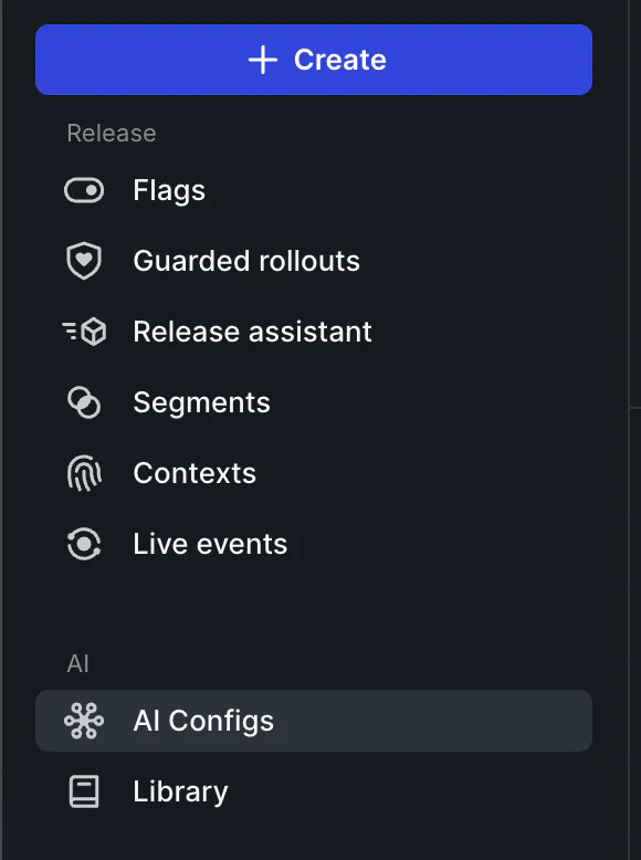
Click the Create config button in the top-right corner of the navigation bar, as shown in the figure below, and name it feature-extraction-config.

Create two variations within feature-extraction-config.

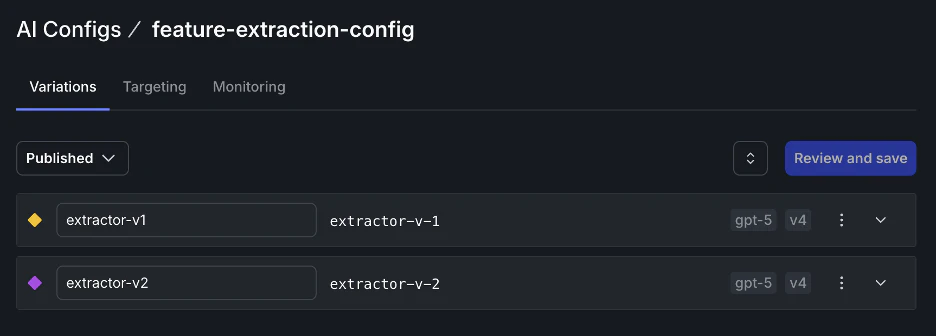
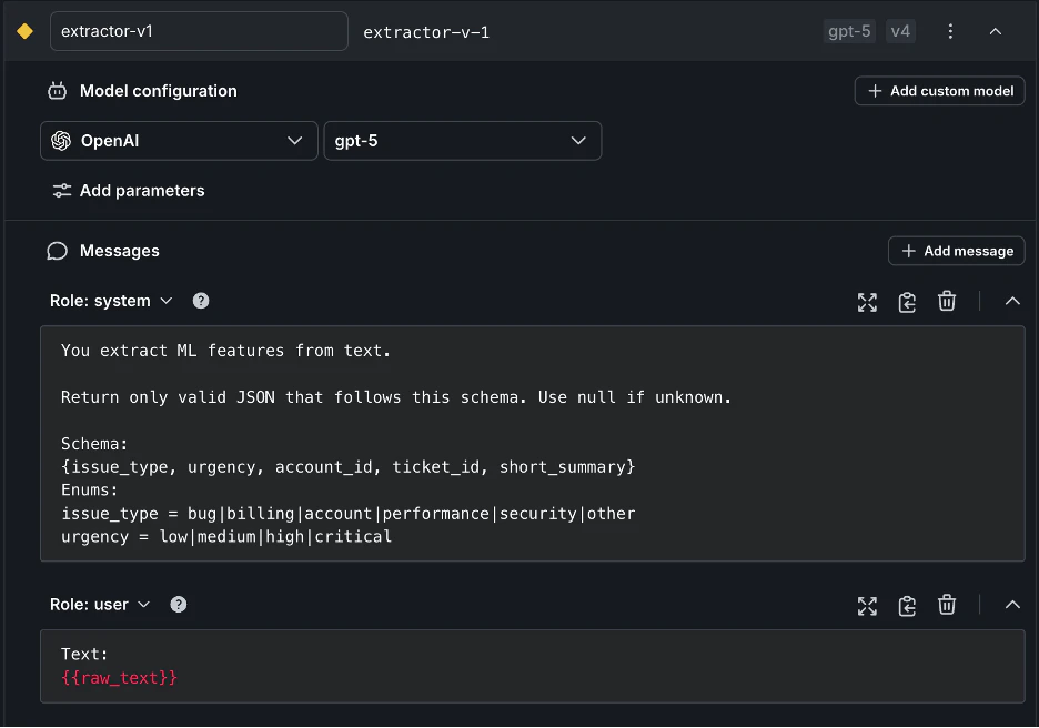
• extractor-v1 (baseline)

• extractor-v2 (candidate): updated prompt wording, stricter schema validation.

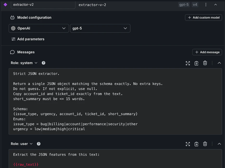
Both variations use the same model, but extractor-v2 applies a stricter contract: It must return a single schema-matching JSON object, with no extra keys, no guessing, verbatim IDs, and a bounded short_summary.

Because prompt and schema changes can affect outputs, latency, and cost, roll out extractor-v2 gradually using LaunchDarkly targeting. A 90/10 split by user key helps the team validate behavior and roll back if needed.

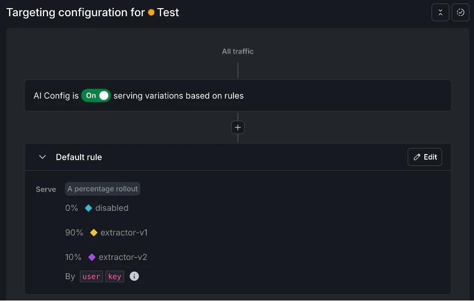
At runtime, your extraction service fetches the config, executes the model call, and records which variation actually ran. The code below demonstrates the workflow.

Note: You can find the following code in the Google colab notebook.

First, import the LaunchDarkly SDK, the LaunchDarkly AI SDK client, and the OpenAI client we will use to run the extraction call.

Next, define a sample support ticket as unstructured input, initialize the LaunchDarkly client and AI client, and set a fallback config in case the config is unavailable.

Next, run the extraction multiple times using different user keys. This allows the 90/10 percentage rollout rule to assign some requests to extractor-v2 while most continue to use extractor-v1. Log the served variation and parse the extracted JSON.

Finally, LaunchDarkly config monitoring helps you compare the operational impact of v1 vs v2, including tokens in/out, requests, errors, and estimated cost.

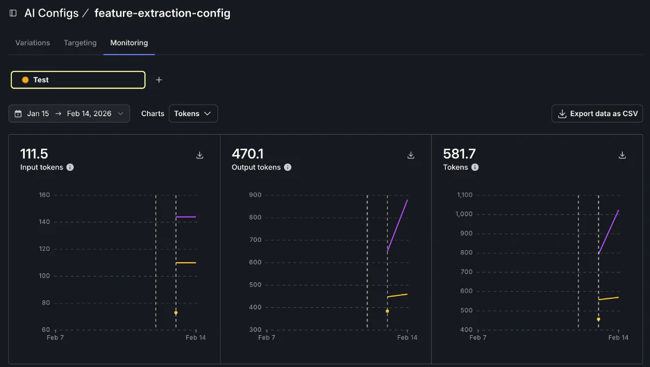
The distribution of rollouts can also be seen in the Monitoring tab (54 requests served by v1 and 6 by v2), and differences in the number of tokens, cost, and error rate can be immediately observed.

Through LaunchDarkly SDKs and integrations, engineers can observe how configuration changes are applied in production, including which variations are served and to which cohorts. When combined with existing ML evaluation, observability, and monitoring systems, this visibility helps supports safer iteration on inference-time behavior and LLM-based feature generation, particularly in online and real-time systems such as recommendations, ranking, and LLM-powered applications.

Real-time ML and LLM systems: how flags map naturally to Configs

LLM-powered pipelines often modify behavior at inference time that is hard to address with static configuration. In LLM-driven pipelines, runtime controls may govern prompt templates, model or provider switching, safety filters and guardrails, cost controls, and LLM-based feature extraction from unstructured inputs.

A concrete example is using an LLM to extract structured features at runtime, where prompt logic and extraction schemas can be updated and evaluated more safely through runtime controls, as shown in the LaunchDarkly LLM data extraction pipeline tutorial. Here’s some example pseudocode:

Make experiments reproducible with logging and versioning

Too many runtime switches can make experiments difficult to reproduce and obscure which configuration was actually executed. To maintain reproducibility, the served configuration should be logged as part of the prediction record. This typically includes the flag or configuration values used, the feature set or prompt version applied, the model version and any key thresholds, and the cohort assignment or rollout percentage associated with the request.

Conclusion

Feature engineering remains one of the most vital and enduring skills in machine learning. It involves transforming raw data into structured, high-value inputs, which is essential for creating reliable models in a production environment. In addition to the establishment of new variables, it also involves the construction of reproducible pipelines, consistency between training and inference, and constant monitoring of the quality of features as data changes.

Combining the practice of disciplined feature engineering with controlled, inference-time experimentation with tools such as LaunchDarkly can help teams safely experiment with the use of features, measures generated by LLM, and model configurations in production. This allows systems to keep in time with varying data and operating conditions with limited risk to model performance and overall system stability.